In a previous post we have given an non-formal introduction to Reinforcement Learning by means of an example. In what follows, we would like to consolidate some ideas and proceed with a more rigorous explanation about what actually Reinforcement Learning is.

In the Reinforcement Learning (RL) framework, the agent makes its decisions as a function of a signal from the environment called the environment’s state. Exploiting a property of the environment and its states, namely the Markov property, the mathematical formalism behind Reinforcement Learning can be described by Markov Decision Processes. To be more thorough, the Markov Decision Processes are the appropriate framework for RL problems with a fully observable environment (all relevant information about the environment are available to the agent).

The understanding of the theory behind Markov Decision Processes is an essential foundation for extending it to the more complex and realistic cases which don’t fit into the Markov formalism.

Markov Processes

A stochastic process $(S_t)_{t\in T}$ is a family of random variables indexed by a set of numbers (called index set), which take values from a set $\textbf{S}$ called the state space. The index set does not need to be a countable set.

Markov processes are stochastic processes used to model systems that have a limited memory of their past. As an example, in population growth studies, the population growth of the next generation depends only on the present population and probably last few generations. A particular case is the first-order Markov process, which is a stochastic process with the conditional probability distribution of future states depending only upon the present state. This property of states is called Markov property.

Markov processes can be classified in:

• Discrete time processes ($T = \mathbb{N}$), also called Markov chains - e.g. Random walk, PageRank- the algorithm Google uses to prioritize the search results, games like go, chess, and many others
• Continuous time processes ($T = [0,\infty)$ ) - e.g. Brownian motion, Birth-death process

In Markov processes one needs to define the transition mechanism between states, which is known in the literature as the Markov kernel. For the discrete-time case (Markov chains), the Markov kernel is known under a more familiar term, the transition matrix or stochastic matrix.

For our goal, that of describing the formalism for sequential decision making problems, the processes of interest are Markov chains.

Markov Chains

To keep the mathematical formulation simple, we concentrate further on Markov chains with a finite state space $\textbf{S} = \{s_1, s_2,\dots, s_N\}$. This enables us to work with sums and probabilities rather than integrals and probability densities. However, the arguments can be easily extended to include continuous state spaces.

A stochastic process $(S_t)_{t\in\mathbb{N}}$ on $\textbf{S}$ has the Markov property if

$$\mathbb{P}[S_{t+1}|S_t] = \mathbb{P}[S_{t+1}|S_1, S_2, ..., S_t].$$

Changing from state $s_i$ at time $t$ to $s_j$ at time $t+1$ is given by the transition probability:

$$P_{ij} := \mathbb{P}[S_{t+1} = s_j|S_t = s_i].$$

In the above formula it is assumed that the transition probabilities do not change with time, they are time-homogeneous (which makes sense in many situations, think of a chess game, the rules of the game don’t change in time):

$$\mathbb{P}[S_{t+1} = s_j|S_t = s_i] = \mathbb{P}[S_{2} = s_j|S_1 = s_i],\; s_i, s_j\in\textbf{S}.$$

The transition matrix/stochastic matrix is

$$\begin{array}{cr} \textbf{P} = \left[\begin{array}{cccc} P_{11}& P_{12} & \dots & P_{1N}\\[2mm] P_{21} & P_{22} & \dots & P_{2N}\\[2mm] \vdots&\vdots&\ddots&\vdots \\[2mm] P_{N1}& P_{N2}& \dots& P_{NN} \end{array} \right] & (1) \end{array}$$

where $P_{ij}, \; (i,\; j = 1, \dots, N)$ are transition probabilities.

The $i-$th row of $\textbf{P}$ gives the distribution of the values of $S_{t+1}$ when $S_t = i$ and hence, $\sum_{j = 1}^N P_{ij} = 1, \;\textrm{for all } i = 1, \dots, N.$

Example basketball game

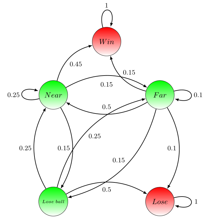
Think of a basketball game with only 2 players played on one half of the basketball field and which finishes when one of the players scores first. There is no time limit and no abandon. It is possible to describe the evolution of one player (let’s say Player1) during such a game as a Markov chain with the following states: $\textrm{Far}$ (has the ball outside 3-point line), $\textrm{Near}$ (has the ball inside 3-point line), $\textrm{Lose ball}$ (the opponent has the ball), $\textrm{Win}$ (Player1 scores), $\textrm{Lose}$ (the opponent scores). It is clear that for a basketball game in general, the Markov property is satisfied, since it is not important for what will happen next what were the previous movements before present situation. In this case there are two states which define the stopping of the game: $\textrm{Win}$ and $\textrm{Lose}$.

Now let’s assume that we have watched several games of Player1 against other opponents and we checked the situation of the games every 30 seconds. From the observations we could say that in $10\%$ of the situations the player starting behind the 3-point line remained there and in $50\%$ of the cases he managed to get close to the basket, in $15\%$ of the cases he has lost the ball behind the 3-point line, in other $15\%$ of the times he scored from the 3-point line and in $10\%$ of the cases he lost the game in a next move after being outside the 3-point line (this could mean that in 30 seconds time the opponent has stolen the ball and managed to score). These percentage values describe the probabilities of transitioning from state $\textrm{Far}$ to every other state in the next time step (as mentioned, the time step is 30 seconds). In a similar way we could determine transition probabilities between every two states from the state space and get the following transition matrix:

$$\begin{array}{cccc} & \begin{array}{ccccc} \textrm{Far} & \textrm{Near}&\textrm{Lose ball}&\textrm{Win}&\textrm{Lose}\end{array} & & \end{array}$$ $$P = \left[\begin{array}{ccccc} 0.10 & 0.50& 0.15 & 0.15 & 0.10\\[2mm] 0.15 & 0.25 & 0.15 & 0.45 & 0 \\[2mm] 0.25 & 0.25 & 0 & 0 & 0.5 \\[2mm] 0 & 0 & 0 & 1 & 0 \\[2mm] 0 & 0 & 0 & 0 & 1 \end{array} \right] \begin{array}{l} \textrm{Far}\\[2mm] \textrm{Near}\\[2mm] \textrm{Lose ball}\\[2mm] \textrm{Win}\\[2mm] \textrm{Lose}\end{array}$$

For this Markov chain we have the following graph representation :

We can take some sample episodes starting in state $S_t = \textrm{Far}$ and going through the Markov chain until we reach any of the terminal states $\textrm{Win}$ or $\textrm{Lose}$ (which mark the end of the game):

• Sample: $\textrm{Far, Near, Win}$ (the player is outside the 3-point line, moves inside the 3-point line, scores)
• Sample: $\textrm{Far, Near, Lose ball, Far, Near, Win}$ (the player starts outside the 3-point line, moves inside the 3-point line, loses the ball and the opponent has to go outside the 3-point line, the player gets the ball back, comes near the basket, scores)
• Sample: $\textrm{Far, Lose ball, Lose}$ (the player is outside the 3-point line, loses the ball, and the opponent scores)

If the state at the present time is $S_t = \textrm{Lose ball}$, we could have some sample episodes like:

• Sample: $\textrm{Lose ball, Lose}$
• Sample: $\textrm{Lose ball, Near, Far, Near, Win}$

At this point the player jumps from state to state according the dynamic of the Markov chain, without knowing which state was good and which was bad. So what we do next is to hire a trainer which knows how good a certain situation is and stimulates the player to reach that situation (state).

Markov Reward Processes (MRP)

In a Markov chain there is no goal, just a jump from state to state according to the transition probability. Now we would like to go a step further with the formalism behind reinforcement learning and introduce the notion of reward, which is the most important ingredient needed to set goals.

Let’s consider a function $r:\textbf{S}\rightarrow\mathbb{R}$ which assigns to a state $s$ a real number $r(s),$ called reward. At each time time step $t$ the reward value is denoted $r_{t+1} := r(S_t),$ where $(S_t)$ is a Markov chain. Now, we define the expected reward function $R:\textbf{S}\rightarrow\mathbb{R}$ as the expected immediate reward from state $s$:

$$\begin{array}{cr}R(s) = \mathbb{E}[r_{t+1}|S_t = s] & (2) \end{array}$$

The expected immediate reward tells us how good or bad it is to be in a state, or, how much reward is hoped to be made from the actual state at the next time step.

Markov chains equipped with expected reward function are called Markov reward processes. Formally, they are defined as the tuple $(\textbf{S},\textbf{P},R, \gamma)$ with

• $\textbf{S}$ a finite countable set (state space)
• $\textbf{P}$ transition matrix defined in $(1)$
• $R:\textbf{S}\rightarrow\mathbb{R}$ reward function defined in $(2)$
• $\gamma \in [0,1]$ a discount factor

Example basketball game as MRP

For the basketball example we could associate to each state the following rewards:

$$r(\textrm{Far}) = r(\textrm{Near}) = 0,\; r(\textrm{Lose ball}) = -0.5,\; r(\textrm{Win}) = +1,\; r(\textrm{Lose}) = -1$$

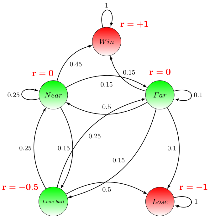
Let’s now denote the vector of rewards $\textbf{r}:=(r(\textrm{Far}), r(\textrm{Near}), r(\textrm{Lose ball}), r(\textrm{Win}),r(\textrm{Lose}))^T$, then the corresponding expected reward (for making only one jump) for the given states can be obtained by multiplying the transition matrix $\textrm{P}$ with the reward vector $\textrm{r}$:

$$R(\textrm{Far}) = -0.075, \; R(\textrm{Near}) = 0.375,\; R(\textrm{Lose ball}) = -0.5, \; R(\textrm{Win}) = 1, \; R(\textrm{Lose}) = -1.$$

In many applications it is not enough to consider only immediate expected rewards to decide how good or bad a state is to be in (e.g. in a chess game one has to go several steps in the future to see what is the potential of a certain state), but to take a cumulative reward on the long run, called the return. In fact the expected return is what we need, but first we will clarify how the return is defined.

Return

The return is defined as some function of the reward sequence $(r_t)_{t\in\mathbb{N}}$ and in the simplest case is the following sum:

$$G_t = r_{t+1} + r_{t+2} + ... + r_{T},$$

where $T$ is a final time step. This notion of return makes sense in problems which can naturally be described in episodes (called episodic tasks), such as playing a game of chess. In such applications, the final state can be reached in a finite number of steps. What about when this is no longer the case? What is the situation of continuing tasks, applications which are not episodic, such as learning a certain theory from the internet (this could go on infinitely, there is no stop and start again from the beginning), or controlling a dynamical process? In these cases it no longer makes sense the above defined return, since the final time step would be $T = \infty$ and the sum could also be infinite(e.g. at each time step the reward is a positive number $\alpha > 0$). That is why, another return is introduced, the discounted return

$$\begin{array}{cr} G_t = r_{t+1}+\gamma r_{t+2} + \gamma^2r_{t+3} + ... = \sum_{k=0}^{\infty}\gamma^k r_{t+k+1}, & (3)\end{array}$$

where $\gamma \in [0,1]$ is the discount term.

Now, what is the idea behind this apparently complicated formulation? First of all it is important to notice that the above infinite series converges (has a finite sum) if the sequence of rewards $(R_{t+k+1})_{k\in\mathbb{N}}$ is bounded (there exists a number $M > 0$ such that $M \geq |r_{t+k+1}|,\;\textrm{ for all }\; k\in\mathbb{N}$) and $\gamma < 1:$

$$\sum_{k=0}^{\infty} \gamma^kr_{t+k+1}\leq |\sum_{k=0}^{\infty} \gamma^kr_{t+k+1}| \leq M \sum_{k=0}^{\infty} \gamma^k = M\frac{1}{1-\gamma},$$

where $\sum_{k=0}^{\infty} \gamma^k$ is the well-known geometric series.

It is clear that when $\gamma = 1$ the infinite series $(3)$ converges if and only if there exists a position $T > 0$ such that $r_t = 0,$ for all $t > T$. In other words, the definition of the return with $\gamma = 1$ makes sense for the finite case or for the infinite case with null reward from a certain time step $T$ further.

Another reason to use a discount term is to decide how important should future rewards be. For values of $\gamma$ close to $0$, the interest is in immediate rewards, whereas for $\gamma$ close to $1$ also future rewards are taken more strongly into account. Humans have a preference for immediate rewards, but this is not always effective, take the example of a chess game where it is important to have a longer term strategy instead of following only to get maximum reward at each step (it makes sense sometimes even to give up on an important piece at some point having in mind a winning position after some steps).

The discount factor also accounts for the uncertainties in the future.

Example basketball game returns

For some sample episodes in our basketball example we compute the returns. Assume that we start in the state $S_1 = \textrm{Far}$ and take a discount factor $\gamma = \frac{1}{2}$, then we get:

• Sample: $\textrm{Far, Near, Win}$

$$G_1 = \sum_{k=0}^{\infty} \gamma^{k}r_{k+2} = 0 + \frac{1}{2}\cdot 0+ \frac{1}{4}\cdot 1+ \frac{1}{8}\cdot 1 + \frac{1}{16}\cdot 1 + ... = \frac{1}{2}$$

• Sample: $\textrm{Far, Near, Lose ball, Far, Near, Win}$

$$G_1 = \sum_{k=0}^{\infty} \gamma^{k}r_{k+2} = 0+ \frac{1}{2}\cdot 0+ - \frac{1}{4}\cdot 0.5 + \frac{1}{8}\cdot 0 + \frac{1}{16}\cdot 0 + \frac{1}{32}\cdot 1 + \frac{1}{64}\cdot 1 + ... = -\frac{1}{16}$$

• Sample: $\textrm{Far, Lose ball, Lose}$

$$G_1 = \sum_{k=0}^{\infty} \gamma^{k}r_{k+2} = 0-\frac{1}{2}\cdot 0.5 - \frac{1}{4}\cdot 1 - \frac{1}{8}\cdot 1 - \dots = -\frac{3}{4}$$

Please notice that in the way we have defined the rewards for the basketball example, the process will not stop when first reaching “Win” or “Lose”, but will infinitely come back in these states. It is possible to make this example episodic, by introducing a so-called absorbing state $\textrm{Stop}$ (state with reward $0$ and probability $1$ to jump to itself) and give $1$ probability of transition from $\textrm{Win}$ and $\textrm{Lose}$ to $\textrm{Stop}$. In this way, after reaching one of the states $\textrm{Win}$ or $\textrm{Lose}$, the reward sequence wil continue infinitely with 0’s.

Value function

The measure for how good a state is on the long term is given by the value function. The Value function of a state $s$ is defined as the expected return starting from state $s\in\textbf{S}$

$$V(s) = \mathbb{E}[G_t|S_t = s]$$

It is possible to rewrite the value function of a state $s$ at the present step $t$ as a sum of the expected immediate return and the value function of the succesor state $S_{t+1}:$

$$\begin{array}{ll} V(s) & = \mathbb{E}[G_t|S_t = s]\\[2mm] & = \mathbb{E}[r_{t+1} + \gamma r_{t+2} + \gamma^2 r_{t+3} + ...|S_t = s]\\[2mm] & = \mathbb{E}[r_{t+1} + \gamma (r_{t+2} + \gamma r_{t+3} + ...)|S_t = s]\\[2mm] & = \mathbb{E}[r_{t+1} + \gamma G_{t+1}|S_t = s]\\[2mm] & = \mathbb{E}[r_{t+1} + \gamma V(S_{t+1})|S_t = s] \end{array}$$

Bellman equation

This is in fact the Bellman equation for MRP and in the following we will show how to compute the value function of the states. Consider the state space $\textbf{S} = \{s_1,\dots, s_N\},$ then the Bellman equation

$$\begin{array}{ll}V(s_i)& = \mathbb{E}[r_{t+1} + \gamma V(S_{t+1})|S_t = s]\\[2mm] & = R(s) + \gamma \sum_{s_j\in\textbf{S}} P_{ij}V(s_j) \end{array}$$

can be written in matrix form as:

$$\left[\begin{array}{c} V(s_1)\\[2mm] V(s_2)\\[2mm] \vdots\\[2mm] V(s_N)\end{array}\right] = \left[\begin{array}{c} R(s_1)\\[2mm] R(s_2)\\[2mm] \vdots\\[2mm] R(s_N)\end{array}\right] + \gamma \left[\begin{array}{cccc} P_{11}& P_{12} & \dots & P_{1N}\\[2mm] P_{21} & P_{22} & \dots & P_{2N}\\[2mm] \vdots&\vdots&\ddots&\vdots \\[2mm] P_{N1}& P_{N2}& \dots& P_{NN} \end{array} \right] \left[\begin{array}{c} V(s_1)\\[2mm] V(s_2)\\[2mm] \vdots\\[2mm] V(s_N)\end{array}\right]$$

If we denote and let $\textbf{v} := (V(s_1) \; V(s_2)\;\dots\;V(s_N))^T$ and $\textbf{R}:= (R(s_1) \;R(s_2)\;\dots\; R(s_N))^T$, then we have the following shorter notation:

$\textbf{v}=\textbf{R}+\gamma\textbf{P}\textbf{v}$ which brings to

$$(\textbf{I}-\gamma\textbf{P})\textbf{v} = \textbf{R},$$

where $\textbf{I}$ is the identity matrix. The Bellman equation has a unique solution when $\gamma \neq 1.$ When $\gamma = 1$, the matrix $(\textbf{I}-\gamma\textbf{P})$ is degenerated, since the transition matrix has $1$ as eigenvalue. In this case, there is no unique solution of the equation.

Solving the linear system is of order $O(N^3)$, where $N$ is the number of states, so direct solution is possible for small MRP. For large MRP there are different iterative approaches such as Dynamic Programming, Monte-Carlo evaluation, Temporal-Difference learning.

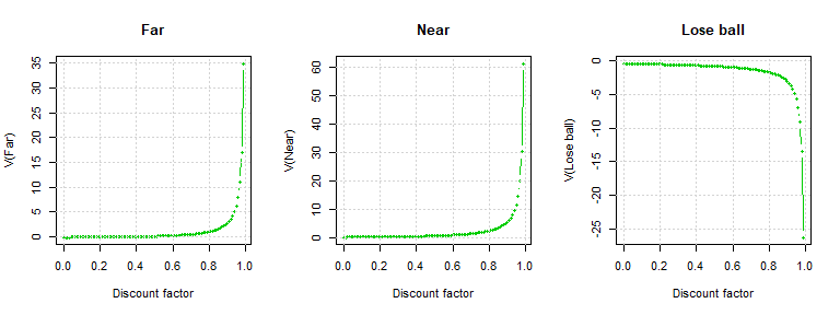
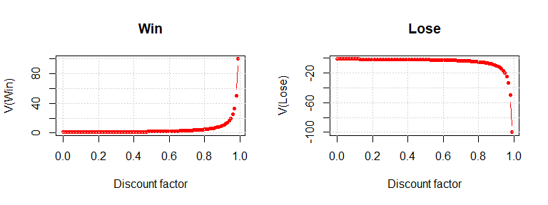
Example basketball game compute value function

By varying the discount factor $\gamma$ in the interval $[0,1)$, we display the evolution of the state values. One can see that the values of the states which show that Player1 is in control of the ball ($\textrm{Far, Near, Win}$) increase as the discount factor increases and the other states, which have a negative reward ($\textrm{Lose ball, Lose}$) decrease as the discount factor increases. The curves for the state values increase/decrease exponentially (are unbounded) as $\gamma$ goes to $1$. However, by introducing the absorbing state $\textrm{Stop}$ (mentioned before), they will stabilize to a value.

So far, the player has learned which situations could bring to a win and which to a lose, but he still cannot decide how to act in a game. Further, we want to give the player this possibility as well, and let him decide how to approach the game, hoping that the trainer showed him (by the value function) what he has to know in order to win a game.

Markov Decision Processes (MDP)

At each time step $t$ in a Markov chain $(S_t)$ over $\textbf{S}$ we have a reward $r_t:= r(S_t)\in\mathbb{R}$. A Markov decision process is formally defined as the tuple $( \textbf{S} , \textbf{A} , \textbf{P} , R, \gamma)$ with

• $\textbf{S} = \{s_1, s_2,\dots, s_N\}$ a finite set of states,
• $\textbf{A}$ a finite set of actions
• $\textbf{P}$ defined by the transition probabilities $P_{ss'}^a = \mathbb{P}[S_{t+1} = s'|S_t = s, A_t = a],$ which gives the probability that taking action $a$ in state $s$ at moment $t$ will lead to state $s'$ at moment $t+1$.
• $R:\textbf{S}\times\textbf{A}\rightarrow\mathbb{R}$ a reward function
  $R(s,a) = \mathbb{E}[r_{t+1}|S_t = s, A_t = a]$ is the expected immediate reward that the agent receives when changing from state $s$ by taking the action $a$.
• $\gamma$ a discount factor ($\gamma \in [0, 1]$)

In the Markov reward processes we didn’t have any action, we had transition between states and values for the states in the form of rewards. By giving the player the chance to take a certain action when being in a state, the player will make a strategy for the game, called policy. His goal now will be to find the policy which helps him win, in mathematical formalism, the optimal policy.

Policy

A policy $\pi$ assigns to each state $s\in \textbf{S}$ a probability distribution $\pi_s$ on the set of actions $\textbf{A}$ $\pi(a|s):=\pi_s(a).$ Once we have defined a policy $\pi$, the Markov decision process becomes a Markov reward process with the state space $\textbf{S}\times\textbf{A}.$ For the basketball example this could mean that after having a strategy, the game developes as a sequence of states and associated actions.

In this setting (with fixed policy $\pi$), we have to specify how the transition mechanism between the states in the state space $\textbf{S}\times\textbf{A}$ looks like. If at time step $t$ we are in $(S_t,A_t)=(s,a)\in\textbf{S}\times\textbf{A}$, the transition at time $t+1$ to $(s',a')\in\textbf{S}\times\textbf{A}$ is given as:

$$P_{ss'}^a \cdot\pi(a'|s').$$

The expected immediate reward for being in a state $(s,a)\in\textbf{S}\times\textbf{A}$ at time step $t$ is

$$R(s,a)\cdot\pi(a|s)$$

Value Function

We can define the state-value function $V_{\pi}(s)$ of an MDP as the expected return starting from state $s$ and following policy $\pi$:

$$V_{\pi}(s) = \mathbb{E}[G_t|S_t=s]$$

State-value function is a measure that tells us how good it is to be in state $s$ by further following policy $\pi$.

The action-value function $Q_{\pi}(s,a)$ is the expected return starting from state $s$, taking action $a$, and following policy $\pi$:

$$Q_{\pi}(s,a) =\mathbb{E}[G_t|S_t=s, A_t=a].$$

The action-value function tells us how good is it to take a certain action when being in a certain state.

The core problem of Markov decision processes is to find a policy for the agent, the one who makes the decisions. In fact, the goal is to find a policy which maximizes the state value function $V_{\pi}$. For the basketball example, this means to find the best strategy for the game.

Define the pointwise maximum of $V_\pi$ by $V^{*}$, i.e.

$$V^{*}(s) = \max_{\pi} V_\pi(s), \;\textrm{for all}\; s\in\textbf{S}$$

Similarly, the optimal action-value function is defined as

$$Q^{*}(s,a) = \max_{\pi} Q_{\pi}(s,a),\;\textrm{for all}\; (s,a)\in\textbf{S}\times\textbf{A}$$

The function $V^*$ is called the optimal value function and it satisfies the Bellman optimality equation

$$V^*(s) = \max_{a\in \mathcal{A}} \left(R(s,a) + \gamma \sum_{s'\in \mathcal{S}} p_{(s,a),s'} V^*(s')\right), \quad s\in \mathcal{S}.$$

The question we need to ask if there exists a policy $\pi^*$ such that $V_{\pi^*}=V^*$?

Theorem.

1. There exists an optimal policy $\pi^*$ such that $V_{\pi^*}=V^*$.
2. Any such optimal policy $\pi^*$ also satisfies $Q_{\pi^*}=Q^*$.
3. There is always a deterministic policy $\pi^d$ which is optimal, satisfying

$$\begin{array}{l} \pi^d_{s,a} = 1 \quad \text{if} \quad Q^*(s,a) = \max_{b\in A} Q^*(s,b)\\[2mm]\quad \pi^d_{s,a} = 0, \quad \text{otherwise}.\end{array}$$

For the proof of the theorem we refer to the lecture notes of Ashwin Rao or the blog.

In general, the optimal policy is not uniquely determined, but we always find a deterministic policy by maximizing the action-value function. Finding an optimal policy involves solving the Bellman optimality equation, which is a non-linear equation and with no closed form in general. There are several numerical approaches for solving the Bellman optimality equation, such as Dynamic Programming methods (Value Iteration, Policy Iteration), or methods used for Temporal Difference Learning (like Q-learning and SARSA), which will be covered in our next blog.

References:

[1] Richard S. Sutton and Andrew G. Barto: Reinforcement Learning: An Introduction, 2014
(https://web.stanford.edu/class/psych209/Readings/SuttonBartoIPRLBook2ndEd.pdf)

[2] David Silver: RL Course, 2013
(https://www.youtube.com/watch?v=2pWv7GOvuf0)

[3] Lex Fridman: Introduction to Reinforcement Learning
(https://www.youtube.com/watch?v=zR11FLZ-O9M)

[4] Ashwin Rao: Lecture notes (http://web.stanford.edu/class/cme241/lecture_slides/BellmanOperators.pdf)